In geometry, the stereographic projection is a particular mapping (function) that projects a sphere onto a plane. The projection is defined on the entire sphere, except at one point: the projection point. Where it is defined, the mapping is smooth and bijective. It is conformal, meaning that it preserves angles at which curves meet. It is neither isometric nor area-preserving: that is, it preserves neither distances nor the areas of figures.
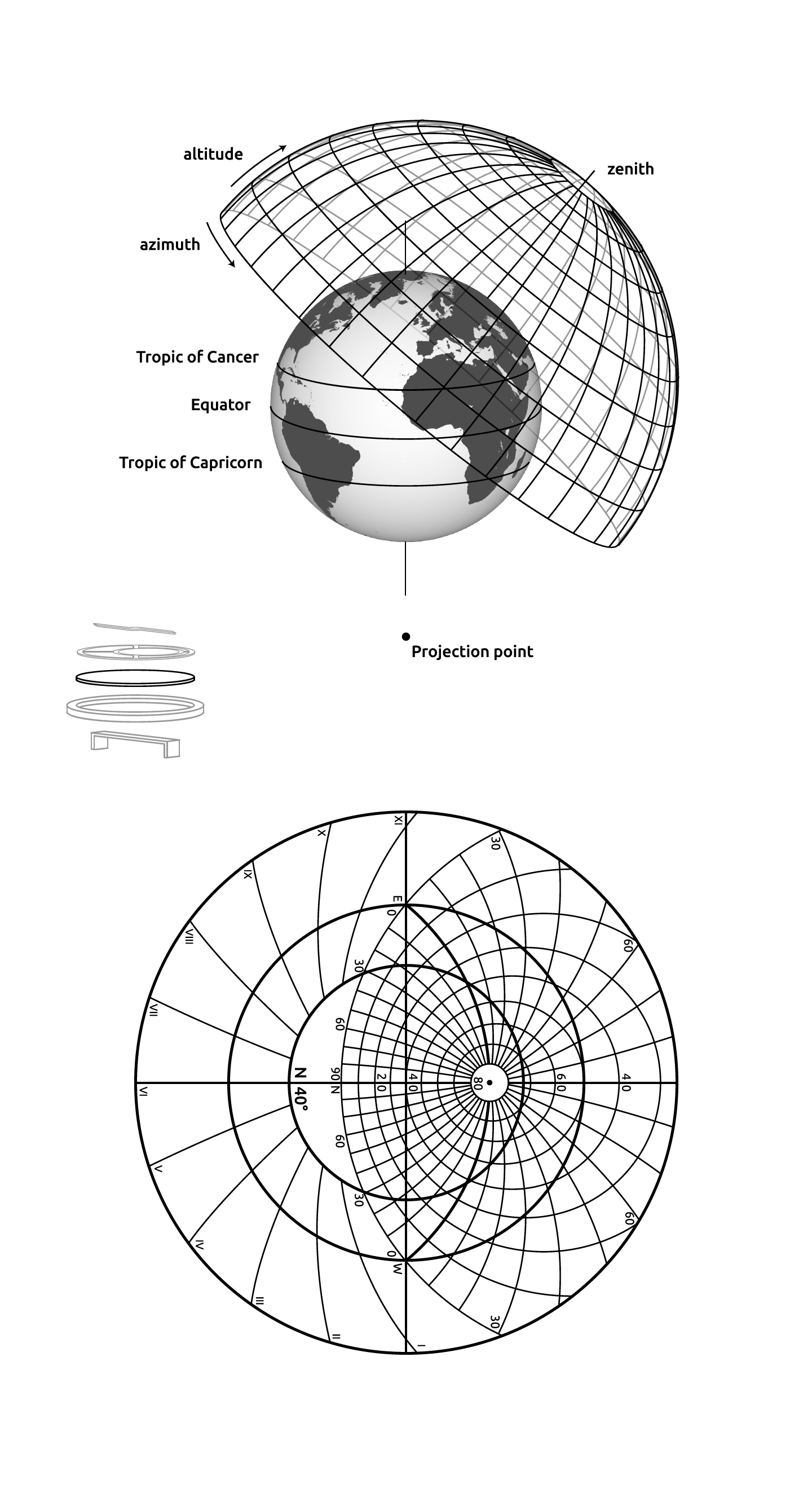
Intuitively, then, the stereographic projection is a way of picturing the sphere as the plane, with some inevitable compromises. Because the sphere and the plane appear in many areas of mathematics and its applications, so does the stereographic projection; it finds use in diverse fields including complex analysis, cartography, geology, and photography. In practice, the projection is carried out by computer or by hand using a special kind of graph paper called a stereographic net, shortened to stereonet, or Wulff net.
A map projection obtained by projecting points P on the surface of sphere from the sphere’s north pole N to point $P^{‘}$ in a plane tangent to the south pole S. In such a projection, great circles are mapped to circles, and loxodromes become logarithmic spirals.
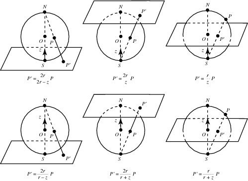
Stereographic projections have a very simple algebraic form that results immediately from similarity of triangles. In the above figures, let the stereographic sphere have radius r, and the z-axis positioned as shown. Then a variety of different transformation formulas are possible depending on the relative positions of the projection plane and z-axis.
The transformation equations for a sphere of radius R are given by
$$
\begin{aligned}
&x=k \cos \phi \sin \left(\lambda-\lambda_{0}\right) \
&y=k\left[\cos \phi_{1} \sin \phi-\sin \phi_{1} \cos \phi \cos \left(\lambda-\lambda_{0}\right)\right]
\end{aligned}
$$
where $\lambda_{0}$ is the central longitude, $\phi_{1}$ is the central latitude, and
$$
k=\frac{2 R}{1+\sin \phi_{1} \sin \phi+\cos \phi_{1} \cos \phi \cos \left(\lambda-\lambda_{0}\right)}
$$
The inverse formulas for latitude $\phi$ and longitude $\lambda$ are then given by
$$
\begin{aligned}
&\phi=\sin ^{-1}\left(\cos c \sin \phi_{1}+\frac{y \sin c \cos \phi_{1}}{\rho}\right) \
&\lambda=\lambda_{0}+\tan ^{-1}\left(\frac{x \sin c}{\rho \cos \phi_{1} \cos c-y \sin \phi_{1} \sin c}\right)
\end{aligned}
$$
where
$$
\begin{aligned}
&\rho=\sqrt{x^{2}+y^{2}} \
&c=2 \tan ^{-1}\left(\frac{\rho}{2 R}\right)
\end{aligned}
$$
and the two-argument form of the inverse tangent function is best used for this computation.
For an oblate spheroid, $R$ can be interpreted as the “local radius,” defined by
$$
R=\frac{R_{e} \cos \phi}{\left(1-e^{2} \sin ^{2} \phi\right) \cos \chi}
$$
where $R_{e}$ is the equatorial radius and $\chi$ is the conformal latitude.
Use of the β and π Methods to Determine Fold Orientation
The orientation of bedding measured at different locations across a fold can be used to determine the attitude of the fold axis and of the axial plane. The readings have introduced these methods. In this article, we will use the following strike and dip measurements of folded beds to illustrate the methods:
110°/40°SW 150°/45°SW
080°/40°SE 040°/50°SE
005°/70°SE 050°/45°SE
132°/60°SW
The β-diagram
On a new overlay, plot the fold limb orientations as planes.
Mark each intersection between planes with a point. If more than two planes intersect at a single location, draw a circle around the point for each additional plane.
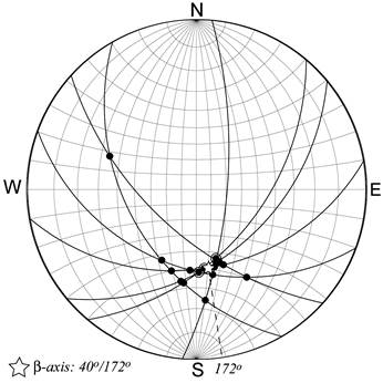
Mark the centre of density of the point distribution. In Figure above (labs), the centre of density is marked with a star. Use the circles to help you to account for the extra “weight” of intersections of more than two planes. One way to think about the weight of points is to imagine each intersection as a small magnet. Where more than two planes intersect, there is an additional magnet for each additional plane. Now imagine that you have a small iron sphere suspended on a string. If you were to hold the sphere just above the centre of the cluster of magnets, each magnet would exert a force on the sphere; magnets located closer together would have a stronger pull on the sphere than a single magnet by itself. Therefore, the suspend sphere might be pulled more to one side than another. The centre of density of the point distribution is the point above which the sphere would come to rest.
The centre of density on a β-diagram is referred to as a β-axis. It is an estimate of the orientation of the fold axis. In our example, the β-axis has an orientation of 40°/172°.
The π-diagram
On a new overlay, plot the poles to the fold limb orientations.
Rotate the overlay until you find the great circle that best fits the set of poles. If the fold measurements are correct, your plotting is correct, and the fold is perfectly cylindrical, then all of the poles should fall on a single great circle. In this example, however, this is not the case, so a great circle has been chosen using the following criteria:
Many of the poles fall on the great circle, or very close to the great circle. For poles that do not fall on the great circle, an attempt is made to distribute them as evenly as possible on either side of the great circle. The great circle you choose to fit the poles is called the π-circle. Find the pole to the π-circle. This is called the π-axis. The π-axis for this example is oriented 40°/175°. The π-axis, like the β-axis, is an estimate of the fold axis. Under ideal circumstances, the β-axis you calculate should be the same as the π-axis. This unusual, however, because it is much more difficult to judge the centre of density of a point cluster than it is to fit a curve to a set of points.
The π-diagram can also be used to estimate the orientation of the axial plane. To do this, we use the angle between the fold limbs, called the interlimb angle. The interlimb angle can be estimated from the spread of the poles along the π-circle. In Figure below, the interlimb angle measured through the poles is 105°. (You can measure this by rotating your stereonet until the π-circle lies on a great circle, and then counting off the distance.) Note, however, that there are actually two possible interlimb angles: The other is 75°. To decide which interlimb angle to use requires that you have some additional knowledge about the shape of the fold. If the fold is tightly closed and has an interlimb angle of less than 90°, then you would use 75°. If the fold is less tightly closed, and has an interlimb angle greater than 90°, then you would use 105°.
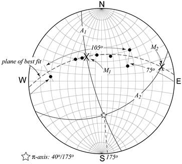
Regardless of which interlimb angle you use, the procedure is the same. First, mark the midpoint (x) of the interlimb angle. Next, rotate your overlay until the midpoint and the π-axis lie on the same great circle, and trace the great circle to find the limb bisectrix, the plane that lies exactly between the limbs of the fold (as represented by your data). The limb bisectrix is an approximation of the axial plane.
If we had independent information that the fold was not tightly closed, then we would choose the great circle connecting the midpoint of the 105° angle ($M_{1}$) and the π-axis. The orientation of the axial plane ($A_{1}$) would be 164°/76°W. This fold could be described as moderately plunging and steeply inclined.
If we knew that the fold was tightly closed, then we would choose the great circle connecting $M_{2}$ and the π-axis. The orientation of the axial plane ($A_{2}$) would be 066°/42°S. This fold could be described as moderately plunging and steeply inclined.
通过球心的面在赤平面上的投影称为大圆,未通过球心的面在赤平面上的投影称为小圆。
由于构造特点各不相同,为了清楚反映构造起见,采用两种不同的投影方法:
一是面的极点图解,即π图解,就是用面的法线作为点来投影,
例如圆柱状褶皱的褶皱面的极点成一个大圆环带通过极点画出最合适的大圆,称为π圆,π圆的极点就是π轴。另一种是面的大圆图解,即β图解,把所测量的每个面作为大圆来投影;
如果将圆柱状褶皱的褶皱面投影,所有大圆轨迹相交于一点,称为β轴,代表褶皱轴的产状。