The fast fourier transform or FFT is without exaggeration one of the most important algorithms created in the last century. So much of the modern technology that we have today such as wireless communication, GPS and in fact anything related to the vast field of signal processing relies on the insights of the FFT.
But it’s also one of the most beautiful albums you’ll ever see. The depth and sheer number of brilliant ideas that went into it is just astounding it’s easy to miss the beauty aspect of the FFT since it’s often introduced in fairly complex settings that require a lot of prerequisite knowledge such as the discrete fourier transform time domain to frequency domain conversions and much more.
The Fast Fourier Transform (FFT) is an efficient $O(N \log N)$ algorithm for calculating DFTs. The FFT exploits symmetries in the $W$ matrix to take a “divide and conquer” approach. We will first discuss deriving the actual FFT algorithm, some of its implications for the DFT, and a speed comparison to drive home the importance of this powerful algorithm.
To derive the FFT, we assume that the signal’s duration is a power of two: $N=2^l$ . Consider what happens to the even-numbered and odd-numbered elements of the sequence in the DFT calculation.
$$\begin{align}S(k) &=s(0)+s(2) e^{(-j) \frac{2 \pi 2 k}{N}}+\ldots+s(N-2) e^{(-j) \frac{2 \pi(N-2) k}{N}}+s(1) e^{(-j) \frac{2 \pi k}{N}}+s(3) e^{(-j) \frac{2 \pi \times (2+1) k}{N}}+\ldots+s(N-1) e^{(-j) \frac{2 \pi(N-2+1) k}{N}} \nonumber \end{align}$$
$$\begin{align}&=s(0)+s(2)e^{(-j)\frac{2\pi k}{\frac{N}{2}}} + \ldots + s(N-2)e^{(-j) \frac{2 \pi\left(\frac{N}{2}-1\right) k}{\frac{N}{2}}} +\left( s(1)+s(3) e^{(-j) \frac{2 \pi k}{\frac{N}{2}}}+\dots+s(N-1) e^{(-j) \frac{2 \pi\left(\frac{N}{2}-1\right) k}{\frac{N}{2}}}\right) e^{\frac{-(j 2 \pi k)}{N}} \end{align}$$
Each term in square brackets has the form of a $\frac{N}{2}$ -length DFT. The first one is a DFT of the even-numbered elements, and the second of the odd-numbered elements. The first DFT is combined with the second multiplied by the complex exponential $e^{\frac{-(j 2\pi k)}{N}}$. The half-length transforms are each evaluated at frequency indices $k \in{0, \ldots, N-1}$. Normally, the number of frequency indices in a DFT calculation range between zero and the transform length minus one. The computational advantage of the FFT comes from recognizing the periodic nature of the discrete Fourier transform. The FFT simply reuses the computations made in the half-length transforms and combines them through additions and the multiplication by $e^{\frac{-(j 2 \pi k)}{N}}$, which is not periodic over $\frac{N}{2}$, to rewrite the length-N DFT. The formula above illustrates this decomposition. As it stands, we now compute two length-$\frac{N}{2}$ transforms (complexity $2 O\left(\frac{N^{2}}{4}\right)$), multiply one of them by the complex exponential (complexity $O(N)$), and add the results (complexity $O(N)$). At this point, the total complexity is still dominated by the half-length DFT calculations, but the proportionality coefficient has been reduced.
Now for the fun. Because $N=2^l$, each of the half-length transforms can be reduced to two quarter-length transforms, each of these to two eighth-length ones, etc. This decomposition continues until we are left with length-2 transforms. This transform is quite simple, involving only additions. Thus, the first stage of the FFT has $\frac{N}{2}$length-2 transforms (see the bottom part of fomula). Pairs of these transforms are combined by adding one to the other multiplied by a complex exponential. Each pair requires 4 additions and 4 multiplications, giving a total number of computations equaling $8\frac{N}{4}=\frac{N}{2}$. This number of computations does not change from stage to stage. Because the number of stages, the number of times the length can be divided by two, equals $\log_2 N$, the complexity of the FFT is $O(N \log N)$.
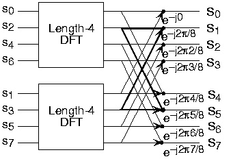
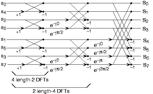
The initial decomposition of a length-8 DFT into the terms using even- and odd-indexed inputs marks the first phase of developing the FFT algorithm. When these half-length transforms are successively decomposed, we are left with the diagram shown in the bottom panel that depicts the length-8 FFT computation.
法国数学家傅里叶提出,任何周期函数都可表示为不同频率的正弦函数和,
或余弦函数之和,其中每个正弦函数和,或余弦函数都要乘以不同的系数,这个和就称为傅里叶级数。
DFT 是指 Discrete Fourier Transform,离散傅里叶变换。
FFT 是指 快速傅里叶变换,它是 DFT 的一种简化计算。
它是根据离散傅氏变换的奇、偶、虚、实等特性,对离散傅立叶变换的算法进行改进获得的。